
“Is my blend homogeneous everywhere, or only where I sample? Is my suspension settling, and from what level of the vessel? When did product A give way to product B?” Three questions about the inside of a volume nobody can see.
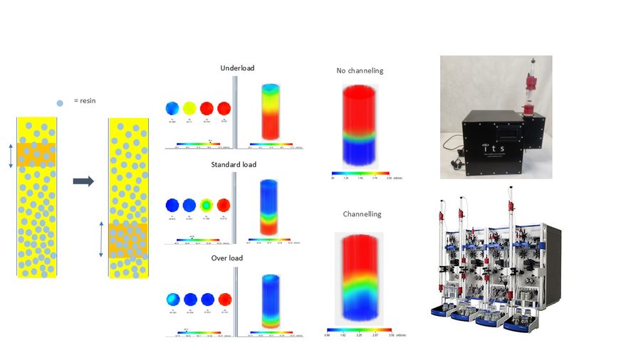
A liquid to liquid blend stopped at forty minutes because that is the instruction written twelve years ago, on equipment that has moved on since.
In a pipe, at a product changeover, the front between old and new product is handled by a purge of fixed duration. Sized long, which is the frequent case, that margin is paid at every changeover, all year.
What the two have in common is the absence of observation inside the volume rather than a lack of measurement precision. No point sensor says what is happening anywhere but where it sits.
In short
Electrical tomography (ECT/ERT) shows where each phase sits across the section of a vessel or pipe, even opaque or metallic, with no calibration for the image. It needs an electrical contrast between the phases. A point spectroscopy says what, at one point: the two combine.
What is actually measured
Electrical tomography does not measure a content directly. It can lead to one, but through a correlation to be established, and that is another subject. Across a straight section of the volume, it measures the distribution of an electrical property of the medium: permittivity for the capacitive variant, conductivity for the resistive one. It then reconstructs an image from it. What you get is a map, not a number. Three consequences follow, and they decide the project.
A section image, not a point
Electrodes set in a belt around the pipe or flush in the vessel wall interrogate the volume step by step. In a sixteen-electrode configuration, a complete set represents 104 independent voltage measurements — that is n(n−3)/2, the count proper to the adjacent strategy in resistance tomography. The systems we implement, those of Industrial Tomography Systems, produce around thirty frames per plane per second. It is this redundancy that makes it possible to reconstruct a distribution where a single sensor would only give a local value.
A contrast, not a composition
The measurement exists if, and only if, the phases present differ electrically. Two liquids of the same conductivity are invisible to each other. It is the contrast, not the composition, that decides feasibility.
A bounded spatial scale
Spatial resolution is about 5 % of the sensor diameter. On a 200 mm pipe, the perceptible detail sits around the centimetre. Enough to see a front, a stratification or a dead zone. Never at the scale of the particle. And it is not the same everywhere in the section: it is better near the electrodes, poorer at the centre.
This family of measurement calls for no chemometric model, neither to build nor to maintain. That is rare, and it changes the whole economics of a project. No design of experiments, no reference sample campaign, no model that ages when the raw material changes supplier. The quantity comes directly from the physics of the measurement and from the reconstruction algorithm.
That does not mean there is nothing to tune. The choice of reconstruction algorithm, for its part, has to be worked on. Fast for real time and progressive gradients, iterative for sharp interfaces, parametric where a process model already exists. Choosing the wrong one smooths out precisely what you were trying to see.
On the distinction between a measurement that requires a model and one that does not: what calibration effort your measurement imposes, and what it costs.
Which technology for which case
A distribution measurement and a point measurement answer different questions. The first says where each phase sits in the section. The second says what sits at one point. Combining them is where the value is.
| Technology | What it follows | Suitable matrices | Calibration burden | Installation | Known condition |
|---|---|---|---|---|---|
| Electrical tomography ECT and ERT | Phase distribution in a section, product front, end of homogenisation | Stirred vessels, pipes, opaque volumes, metal containers | None for the image. A few calibration points where a content is the target | Belt or flush wall electrodes, from 5 mm to 2 m diameter. ATEX certification available | Calls for electrical contrast between the phases. A content is reachable where it governs the conductivity, with temperature compensation |
| MIR spectroscopy | Chemical composition at one point of the circuit | Liquids, viscous and loaded ones included | None where the composition is declared. Full otherwise | Short path length cell, on a recirculation loop | Measures one point of the flow, and the distribution in the volume comes from elsewhere |
| NIR spectroscopy | Content of a constituent, moisture content, identity | Powders, granules, liquids, suspensions | Full most of the time | Immersed probe, window or contact-free measurement | Probes a few milligrams at a time, in one place of the vessel |
The calibration burden column is the one a manufacturer fills in from the technology they make. The known condition column is the one worth asking for.
Where the measurement sits, and why that is the real question
A tomographic sensor observes a plane. Choosing that plane is a process decision, not an instrumentation one, and it is what makes the value of the result.
On a vessel, a low plane sees settling, a high plane sees incorporation and air entrainment, a plane at the level of the impeller sees the shear. None of the three replaces the other two. Two planes also give velocity information, by correlation between successive images. That is how a front is followed.
On a pipe, the question is different. The electrode belt has to be placed where the flow is established, away from a bend, a valve or a pump. A disturbed regime produces a perfectly faithful image of a local disturbance of no interest.
As for the rate, it depends on the configuration. Some systems reach around thirty images per plane per second. Acquiring a complete set of measurements over two planes of sixteen electrodes takes less than a millisecond on fast electronics. These values only make sense in relation to that configuration. The right approach is the reverse: first determine how fast your phenomenon evolves, then check that this rate is reachable.
What is worth preparing on your side
Tomography projects are carried by the mechanics and by the definition of the need, more than by the electronics.
- The service conditions, written. Admissible temperatures and pressures are defined for each installation. They belong to a user requirement specification, with the sensor material, the chemicals in contact and the ranges of each variable factor. Writing that specification before consulting is the best practice of the field.
- The expected electrical contrast between your phases. A conductivity or permittivity measurement on samples of both products answers the main feasibility question in the laboratory, before any commitment.
- Mechanical access and its impact on qualification. A belt fitted to an existing pipe is a simple project. Flush electrodes in a qualified reactor is another, with a requalification costed at scoping.
- The area classification. Where the installation sits in an explosive atmosphere, saying so at the start matters. ATEX certification exists on this family of equipment, and it shapes the configurations available. The texts are directive 2014/34/EU on the equipment side and directive 1999/92/EC on the worker side, with the IEC 60079 series for the equipment.
- A history of durations and purged volumes, changeover by changeover, batch by batch. It is what puts a figure on the gain before any investment.
Conditions for success and limits
The image gives a distribution. A content takes one more step
The image says that a phase occupies such a fraction of such a zone. It does not say by itself that the medium contains 4.2 % of a given constituent. But that extra step is light. Where the quantity sought governs the conductivity of the medium, a few calibration points and a temperature measurement are enough to build a soft sensor that returns a content. It is documented on milk — Sharifi and Young, Food and Bioproducts Processing 90(4), 2012 — and we have implemented it on food-industry effluent. The detail is on the technology page.
The limit therefore moves, it does not disappear: if two different compositions give the same conductivity, no calibration will resolve the ambiguity.
The resolution does not go down to the scale of the particle
About 5 % of the sensor diameter: on a one-metre vessel, the perceptible detail is of the order of five centimetres. You see a cluster, a stratum, an unmixed zone. You do not see an isolated agglomerate of a few hundred microns. The pixel count of the reconstructed image is not published. It is a question to ask, and the answer has to be read against the real diameter of your equipment.
And this single figure hides a non-uniformity you need to know before choosing a plane. The resolution of an electrical tomography is better near the electrodes and poorer at the centre of the section. More counter-intuitive still: increasing the number of electrodes improves resolution near the wall and degrades it at the centre. Yet the centre is often where the dead zone is sought. “About 5 %” is therefore an average order of magnitude, not a guarantee at every point — and the question to ask concerns the resolution at the place that matters to you.
Lucas, Margo, Oussar, Holé, Spatial Resolution in Electrical Capacitance Tomography, 2015, arXiv:1503.01311, open access.
Electrical contrast is what makes the image
Two oils of similar permittivity, two aqueous solutions of identical conductivity: the image will be uniform, and it will not carry the information sought. This point is settled in the laboratory, upstream, for a negligible cost. It is the first trial we ask for, and it is also the one that sometimes leads us to point elsewhere at this stage.
An instrumented plane is still a plane
Tomography corrects the blindness of a point sensor in the observed section, not across the whole volume. A tall vessel with a single plane in the lower third says nothing about the surface. The logic of representative sampling does not disappear: it changes scale.
What it changes, in practice
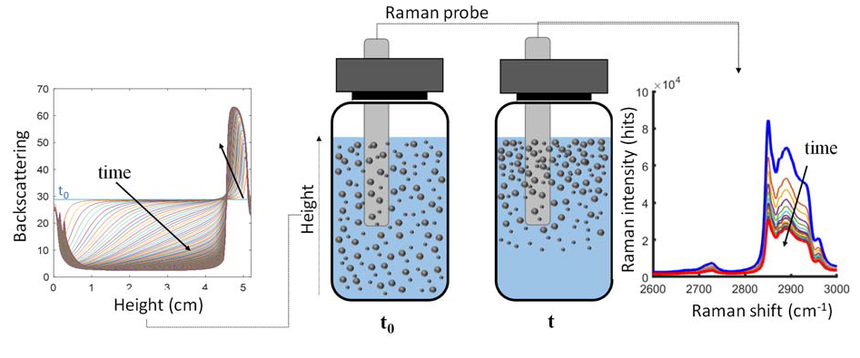
The end of homogenisation is the most direct case. You follow the convergence of the image towards a uniform field, and stop when it no longer moves beyond the noise. It is an endpoint criterion that calls for no absolute calibration. Following a product front in a pipe makes it possible to trigger the valve switch on the material rather than on a timer. Filling is checked by the progression of the level or of the void fraction in a section. Detecting agglomerates, at the scale of the cluster and not of the particle, signals an incomplete dispersion. Following a purification visualises the progression of a front in a bed.
A point of honesty about the evidence available. The published trial on product changeover in a pipe demonstrates the detectability of the front. No cycle gain is quantified in it. It is a solid proof of principle, not a transposable return-on-investment figure. The gain is calculated process by process, on your purged volumes and your real durations. It is the first deliverable of a proof of concept, not a web-page promise.
Frequently asked questions
Can we measure through a metal wall?
Metal is opaque to optical waves, which puts spectroscopic methods through the wall out of reach. Electrical tomography works differently: the electrodes are in contact with the medium or built into the wall, and the information travels through the electric field in the product. A metal container is therefore no obstacle in principle, and its mechanical integration is a real design subject.
Do we have to build a chemometric model?
No. It is one of the rare families of process measurement where the quantity comes out of the physics and the reconstruction, with no reference sample campaign and no model to revalidate. The effort moves to the choice of algorithm, the positioning of the planes and the mechanical integration. The project has a cost, and it simply sits elsewhere.
Can this measurement be used to release a batch?
It steers an operation and documents how it ran. Conformity is established by the tests of the control strategy, since the measurement returns a distribution rather than a composition value. It can enter a documented control strategy as process monitoring data, which is already a great deal for an operation run blind today.
What temperatures and pressures does the sensor take?
Those values are defined for each installation, which is good practice. They follow the sensor material, the chemicals in contact and the configuration chosen, and they are fixed in a user requirement specification, with traceability requirement by requirement and formal approval on both sides. That is the document we start this type of project with.
How long before we know whether it works here?
The electrical contrast question is settled in the laboratory, on a sample, before any installation; the demonstration then follows on a mock-up or a bypass line. Establishing a robust stopping criterion calls for having seen the real variability, several batches, the difficult ones included. A feasibility concluded on a single trial describes that trial.
Describe your vessel or your pipe. You will know whether the distribution is observable.
Forty-five minutes is enough: whether your phases show a usable electrical contrast, where one or two measurement planes should go, what the mechanical integration implies, and what a trial would involve. Some cases call for another route — insufficient contrast, resolution too coarse for what you are looking for, access impossible without requalification: you will then leave with the one that fits.