
“What size are my particles, right now, in the reactor? Has the milling reached the right point? Has my crystallisation finished growing?” Three questions asked about a concentrated medium, whose answer serves during the operation.
That is the paradox of granulometry in a concentrated medium. Classical optical methods call for a medium transparent enough for a photon scattered once to reach the detector without meeting others. Above a certain concentration, that is no longer true: the light is scattered several times, and the result no longer makes sense.
The usual remedy is dilution. Except that a diluted suspension is no longer the suspension in the reactor: equilibria shift, agglomerates come apart, emulsions ripen. The value obtained is right, and it describes the diluted sample.
And meanwhile, the crystallisation carries on, the mill turns, and the decision to stop is taken on a value twenty minutes old.
In short
In concentrated or turbid media, SR-DLS measures a size distribution without dilution or calibration, and picks up the onset of aggregates early. On dry powders and granules, NIR follows a change in particle size by correlation, with a full model.
Depending on your sector: crystallisation of an active ingredient; wet milling and dispersion in chemicals; nanoemulsions and lipid nanoparticles in biopharma.
What is actually measured
A hydrodynamic diameter, not a particle
Dynamic light scattering derives a size from Brownian motion, since a smaller particle moves more. What comes out is the diameter of the sphere that would scatter the same way, solvation included. It is a different quantity from the dimension of an object under a microscope, and the gap is information rather than error.
A distribution rather than a figure
The result is a distribution of sizes. Reducing it to a mean sets aside what usually matters most: a second population, the width, the tail towards the coarse. A process is steered on the shape of the distribution.
Multiple scattering is excluded rather than corrected
That is what makes the measurement possible with no dilution. Resolving the signal in depth identifies the layers where light was scattered once and sets the others aside. The physics is left intact and restricted to the zone where it holds.
The principle in three sentences. A low coherence interferometer associates the scattered signal with the depth it came from, and the coherence length of the source, a few microns, sets how finely that is cut. Spectra are acquired at very high rate, and an inverse Fourier transform draws from them many correlation functions, one per depth slice.
The slices in the multiple scattering regime carry zero weight and the others carry the calculation. That is the whole foundation of measurement with no dilution: what is outside its domain of validity is left out rather than corrected.
Which technology for which case
| Technology | What it follows | Suitable matrices | Calibration burden | Installation | Known condition |
|---|---|---|---|---|---|
| SR-DLS | Size distribution — particles or droplets — from the nanometre to the micron, and the onset of aggregation: scattered intensity rises steeply with size, which makes the measurement sensitive to a small population of large objects well before it becomes the majority | Suspensions, emulsions, concentrated and turbid media, with no dilution | None: the size comes from the physics of the measurement | In-line on a bypass loop, at-line, or through a transparent wall | Calls for laminar flow and freedom from bubbles. Returns neither shape nor surface charge |
| NIR spectroscopy | Variation in particle size, by correlation | Dry powders and granules | Full, always | Probe in contact or contact-free above the flow | The signal also responds to compaction, moisture content and shape |
| Electrical tomography ECT and ERT | Presence of agglomerates, phase distribution | Opaque vessels and pipes | None | Wall electrodes or a fitted belt | Spatial resolution of a few per cent of the diameter, so it works above the scale of the particle |
One point of plain speaking: the second line is correlative. There is no pure spectrum of a particle size. NIR follows a size because size changes how the radiation scatters, which calls for a model calibrated on samples and for that model to be kept alive. Other families exist for dry powders, laser diffraction or focused beam probe counting among them, and they sit outside the nine families covered here.
Two instruments, two results, and both are right
This is the point that occupies the most discussion between a laboratory and a production floor, and it settles in one sentence. A size distribution depends on the basis it is expressed in.
One published case shows it cleanly. On the same injectable lipid emulsion — a 20 per cent intravenous lipid emulsion — two dynamic light scattering instruments return 332 nm and 369 nm — two Zav values, the intensity-weighted mean diameter — a gap of about 11 per cent, easily enough to open an investigation. Converted to a volume distribution, both results become 415 ± 5 nm. The gap was not an instrument fault: the authors attribute it entirely to the optics of the two instruments — 633 nm against 1300 nm of wavelength, 173° against 180° of detection angle — and droplets of that size no longer scatter in the Rayleigh regime but in the Mie regime, where the intensity-weighted Zav depends on exactly those two parameters.
One detail makes the example more instructive still: the two measurements were not made on the same sample. The laboratory instrument measured after a hundredfold dilution in water, the spatially resolved instrument measured the product undiluted. Despite that difference in preparation, conversion to a volume basis reconciles both values at 415 ± 5 nm.
T. Rooimans et al., International Journal of Pharmaceutics 640 (2023) 122960, doi:10.1016/j.ijpharm.2023.122960 — open access. The mechanism in full: two instruments, two figures. And where a specification has to rest on a normative text rather than on common practice, two texts carry it: ISO 22412, Particle size analysis — Dynamic light scattering, and general chapter USP <430>, which transposes it and has been official since 1 May 2024.
The situation is exactly that of transferring a model between two spectrometers, and its solution is documentary rather than technical. The calculation basis, the detection angle and the inversion algorithm belong in the specification, alongside the target value. That is more than good practice: general chapter USP <430> requires them in the test report — laser wavelength, observation angle, and the data analysis program itself, since the result depends on it. Two instruments, two figures.
Where the measurement sits in the process
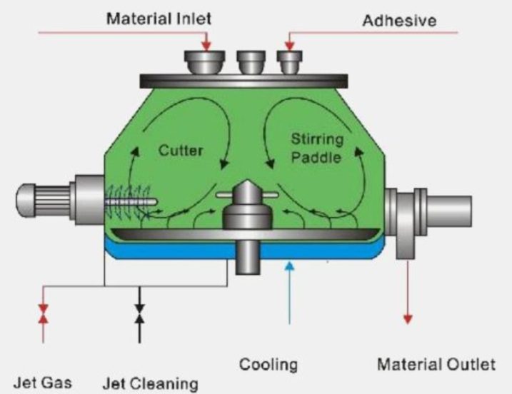
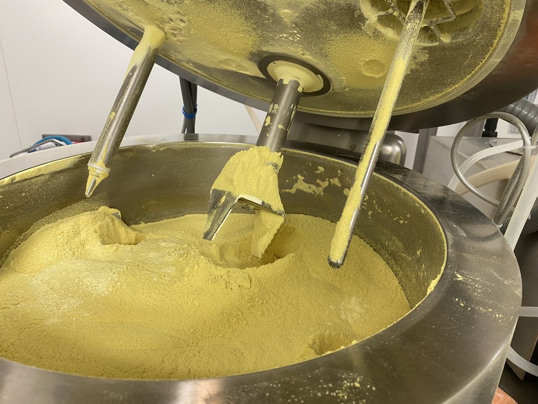
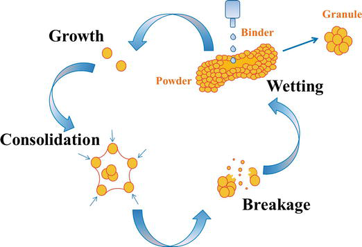
And high shear is not the only route. Wet granulation is also run in a fluid bed, by spraying onto a suspended bed: the same four mechanisms occur, but the material is not worked in the same way and the measurement does not sit in the same place. An illustration of high shear does not stand for both.
| Mode | What it means for a particle size measurement |
|---|---|
| In-line | The probe sits in the reactor or the pipe. The ideal position on paper and the most demanding in practice, since the flow in front of the window has to be controlled, which the inside of a stirred vessel does not always offer |
| On-line, on a bypass loop | A frequent compromise, and often the best. The loop allows the flow rate to be set, the bubbles to be broken and the laminar regime the measurement calls for to be obtained. It adds a transit time to be quantified |
| At-line | Measured beside the line, with no dilution, in minutes. Already a clear gain against sending to a laboratory, and the least demanding way into a first project |
| Off-line | Stays useful as the reference method, on condition that its calculation basis is made explicit, which is what makes the comparison meaningful |
What is worth preparing on your side
- The target size range and the expected width of the distribution. Those two figures decide applicability before anything else.
- The hydraulic conditions available: flow rate, presence of bubbles, viscosity, temperature. Real feasibility is settled here, much more than on the instrument specifications.
- The temperature of the medium at the measurement point, and its stability. A size derived from Brownian motion follows the viscosity and therefore the temperature. A correction is applied, and it calls for knowing the value in the right place.
- The current reference method and its calculation basis. With that in hand, a comparison concludes something. Without it, the trial is judged on a gap that is a convention.
- The area requirements. In standard configuration this family carries no certification for explosive atmospheres; compliant configurations exist, but they are built to order. Where your area calls for it, that is a first question rather than a last one.
Conditions for success and limits
Laminar flow, and freedom from bubbles
The two governing conditions, and they are hydraulic rather than optical. A turbulent flow adds to Brownian motion a displacement that carries no size information, and an air bubble scatters massively. Shear above the diffusion rate of the particles works the same way. Designing the loop is therefore the heart of the project, and it is as much a matter of pipework as of sensor.
The width of the distribution sets what can be read
Above a polydispersity index of 0.3 the default interpretation no longer holds: the result calls for further analysis before it can be read as a distribution. And two populations whose sizes sit closer than a factor of about three are reported together. These are properties of the method rather than of one instrument.
The standing of those two markers is worth stating: they are field rules, not normative thresholds. General chapter USP <430>, which transposes ISO 22412, defines the polydispersity index as a dimensionless measure of the breadth of the distribution — and sets no limit on it. The only published threshold we could attribute is Malvern Panalytical’s: above 0.7 the sample is too broad for DLS to suit it. The factor of three comes from the same publisher as a rule of thumb, the theoretical limit sitting lower.
The promise is about flow, the qualification is about rest
The most interesting gap in this field. Available qualification protocols verify accuracy and precision on a static sample. Performance in flow is what remains to be demonstrated — and it is exactly where an auditor looks. The answer is to build a verification protocol in real conditions, with a control material and a defined periodicity. It is designed rather than supplied.
Always ask what the reference method was
In many application studies in this family, the reference used to validate the measurement is the same instrument in another configuration, which demonstrates reproducibility. Accuracy is established by certified standards or by an independent method with its calculation basis made explicit. The question to put to a supplier, and to us, is what you compared against and with what metrological traceability.
What the method leaves to others, and it is worth knowing early: shape, surface charge and chemical nature. A suspension whose particles agglomerate and one whose particles grow give the same evolution of size. Where that distinction matters to your process, a second measurement supplies it, and it is a typical case of two technologies completing one another.
What it changes, in practice
Three families of process draw a direct benefit from it, and it is measurable.
Crystallisation: following nucleation and growth continuously makes it possible to stop at the target rather than at a fixed duration. And to detect a secondary nucleation at the moment it occurs, not at final testing. Wet milling: it is the clearest example, since the energy spent after the target is reached is entirely lost, and sometimes harmful. Emulsification: the stability of an emulsion reads in the drift of its distribution. Often well before a viscosity or turbidity measurement moves.
In all three cases, the gain is calculated on your history, real durations, rework rates and deviations from specification, during the scoping, before any investment.
Frequently asked questions
Do we really have to give up diluting?
Where your suspension is stable to dilution and the laboratory turnaround suits you, the classical method does the job well and costs less. Measurement with no dilution earns its place when dilution changes the product, or when the decision has to be taken during the operation. Two criteria, and one of them is enough.
Is there a chemometric model to build and to maintain?
For the size measurement itself, no: the quantity comes from the signal processing, out of the physics of Brownian motion. That is a fundamental difference from a spectroscopic content measurement and it changes the economics of the project, with no reference sample campaign and no model to revalidate. That is not merely our reading: general chapter USP <430> states it plainly — sizes obtained by DLS are not relative values calculated from standards of known size but values calculated from first principles, so that calibration cannot be performed. The effort moves to the physical integration, which is where the work sits.
Can we measure through the wall of a reactor?
Through a clean transparent wall, in some configurations, yes. Two points usually decide: fouling of the wall on the product side, and the fact that the measured layer runs along the wall, which is representative of the bulk in some geometries and not in others. A bypass loop stays the more dependable route in the majority of cases.
Is the technology recognised by the authorities?
Dynamic light scattering is an established and standardised method: it is the subject of ISO 22412 and of general chapter USP <430>, harmonised within the Pharmacopoeial Discussion Group and official since 1 May 2024.
Its spatially resolved variant, by contrast, is named in no guidance, no reflection paper and no pharmacopoeial chapter — we looked. It appears in FDA research work on continuous manufacturing, a 2022 symposium and a 2021 poster, both carrying the explicit note that they do not represent the agency’s positions. That is documented interest on the part of the regulator’s own researchers, and nothing more. Recognition of a method is in any case never approval of one instrument.
The distinction is worth holding, because it is what separates an honest citation from a stretched one — and because it decides what you will be able to write in a dossier. What <430> describes is a measurement in a cell, on a diluted and dust-free sample: the chapter asks that concentration be adjusted to rule out multiple scattering, which the in-line measurement achieves by another route. The compendial frame exists for the quantity; it has not yet been written for obtaining it without dilution.
And on a powder, what does the pharmacopoeia already measure?
A great deal, and it is worth knowing before starting an in-line project: the reference exists, it is standardised, and it is what an in-line measurement will have to be reconciled with. The USP technical guide Powder characterization for continuous manufacturing applications lists them.
- <786> Particle Size Distribution Estimation by Analytical Sieving — sizing by sieving, sieve types and agitation modes.
- <811> Powder Fineness — the descriptive classification of fineness, coarse to very fine, from the median dimension.
- <616> Bulk Density of Powders — bulk and tapped density, and what follows from them on compressibility.
- <1174> Powder Flow and <1063> Shear Cell Methodology — angle of repose, Carr index, Hausner ratio, flow through an orifice, shear cells.
- <1097> Bulk Powder Sampling Procedures — the sampling plan, segregation error and sampling method error.
Two markers the guide gives that clear up a specification discussion. Particle size is defined there, after ISO 9276, as the diameter of a sphere having the same physical properties — the same equivalent-sphere reasoning as the hydrodynamic diameter above, and the reason none of these methods returns exactly the same figure. And below roughly thirty microns of median size, surface forces overcome gravity: flowability deteriorates, and that is often where the need to follow size during the operation rather than after it comes from.
USP Technical Guide, Powder characterization for continuous manufacturing applications, © 2025 The United States Pharmacopeial Convention, Rockville, MD — § 2.2.1 and table 1. An informational document: it carries no requirement; the chapters it cites are enforceable under their own conditions. All the texts, and what each governs.
What measurement rate can we expect?
It follows entirely from the configuration: concentration, target size range, integration time chosen, loop flow rate. Figures quoted for this family vary by a large factor with the measurement context, so a rate quoted with its context is the one to work from. The sound approach is to set the rate your process calls for first, then to verify it is reachable in your conditions.
Can we bring the data into our supervision system?
Yes, and it is one of the strengths of this family. A standardised interface exposes the full distribution and many parameters, for reading and for writing, so a third-party sensor can correct the measurement in real time, temperature for instance. Two points to settle early: the security policy of that interface, rarely documented, and a server that accepts writes from third-party clients, which deserves attention in a regulated environment. Data and systems.
Describe your suspension and your flow conditions. That is what decides.
Forty-five minutes is enough to know whether measurement without dilution applies to your medium, what hydraulic configuration it implies, and what a trial would cost. Some cases call for another route — a distribution too broad, unavoidable bubbles, a classified zone: you will then leave with the one that fits.